What an aeromagnetic survey measures
An aircraft or drone carries a magnetometer along parallel flight lines, usually tens to hundreds of metres apart and as low as is safe, and records the strength of the Earth's magnetic field every few metres. Tie lines flown across them let the contractor level the lines to one another. The readings, less the Earth's main field (the model called the IGRF), are gridded into total magnetic intensity, or TMI, in nanotesla (nT).
What the grid maps is magnetic minerals: almost always magnetite, and now and then monoclinic pyrrhotite or maghemite. It does not map rock names. A basalt can read strongly or barely at all depending on how much magnetite it holds, and the same unit changes character where it was altered. Alteration can destroy magnetite, as it often does along shear zones, or create it, as in some skarns and iron oxide copper-gold systems. Weathered cover adds a signal of its own: maghemite in laterite gives a speckled, near-surface texture.
Make the picture before you read it
A grid is numbers. How you colour and light them decides what you see.
- Stretch. A histogram-equalised stretch spreads the colours evenly over the values, so subtle features show everywhere, but it exaggerates small differences. A linear stretch keeps colour in proportion to value, which is what you want when comparing the strength of two anomalies.
- Sun shading. Shading lights the grid as if it were a surface and picks out the gradients that face the light. Structures running parallel to the light fade out, so swing the sun round, or light the grid from several directions at once, before deciding a structure is not there.
- Fit the colours to your ground. A strong body next door can take most of the colour ramp and flatten everything else. Stretching to the area in view, or to your tenement, gives quiet ground the full range.
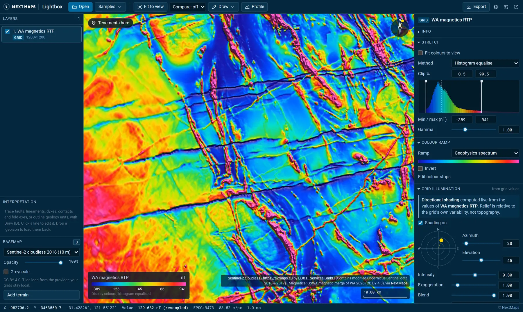
Open this ground prepared for interpretation in Lightbox: Widgiemooltha magnetics. Or open your own grid: it is read in your browser and never uploaded.
Why the anomaly is not over the rock
Except at the magnetic poles, the Earth's field is inclined. A magnetised body in it produces a high paired with a low, and the pair is shifted off the body: the high towards the magnetic equator, the low towards the pole. How far depends on the inclination and on the body's depth and shape. In the Western Australian goldfields, where the field is inclined at about 64 degrees, the high over a shallow, compact body sits close to over it. Where the field is flatter the shift grows: near Geita, in Tanzania, where it is inclined at about 28 degrees, a hole drilled on the high over a small pipe can miss it.
Reduction to the pole (RTP) is a filter that recalculates the grid as if it had been flown at the magnetic pole, where the field is vertical and an anomaly sits over its source. It is the usual grid to interpret from, with two conditions:
- It assumes the rocks are magnetised along today's field. Where they carry a strong magnetisation of their own, the RTP shows the body in the wrong shape or place (see the next section).
- It struggles near the magnetic equator. As the field flattens, bodies that strike magnetic north-south give almost no anomaly, and the filter has to amplify them, noise and all. Within about 20 degrees of the magnetic equator, interpreters use a stabilised RTP, a reduction to the equator or the analytic signal instead, and check each against the others.

In Magnetics for Geologists you drag the field from Kalgoorlie to Bamako and watch this happen, then work real grids both ways.
When the reduced-to-pole grid lies
Many rocks carry a remanent magnetisation, locked in when they cooled or formed, which can point in a very different direction from today's field. Where it is strong it outweighs the induced magnetisation, and an RTP calculated for today's field shows the body in the wrong shape, often as a low or a lopsided pair.
The Widgiemooltha dykes, about 2.4 billion years old, cut east-west across the southern Yilgarn Craton. Many of them carry a remanence opposed to today's field, so on the RTP they read as sharp, straight lows rather than highs.
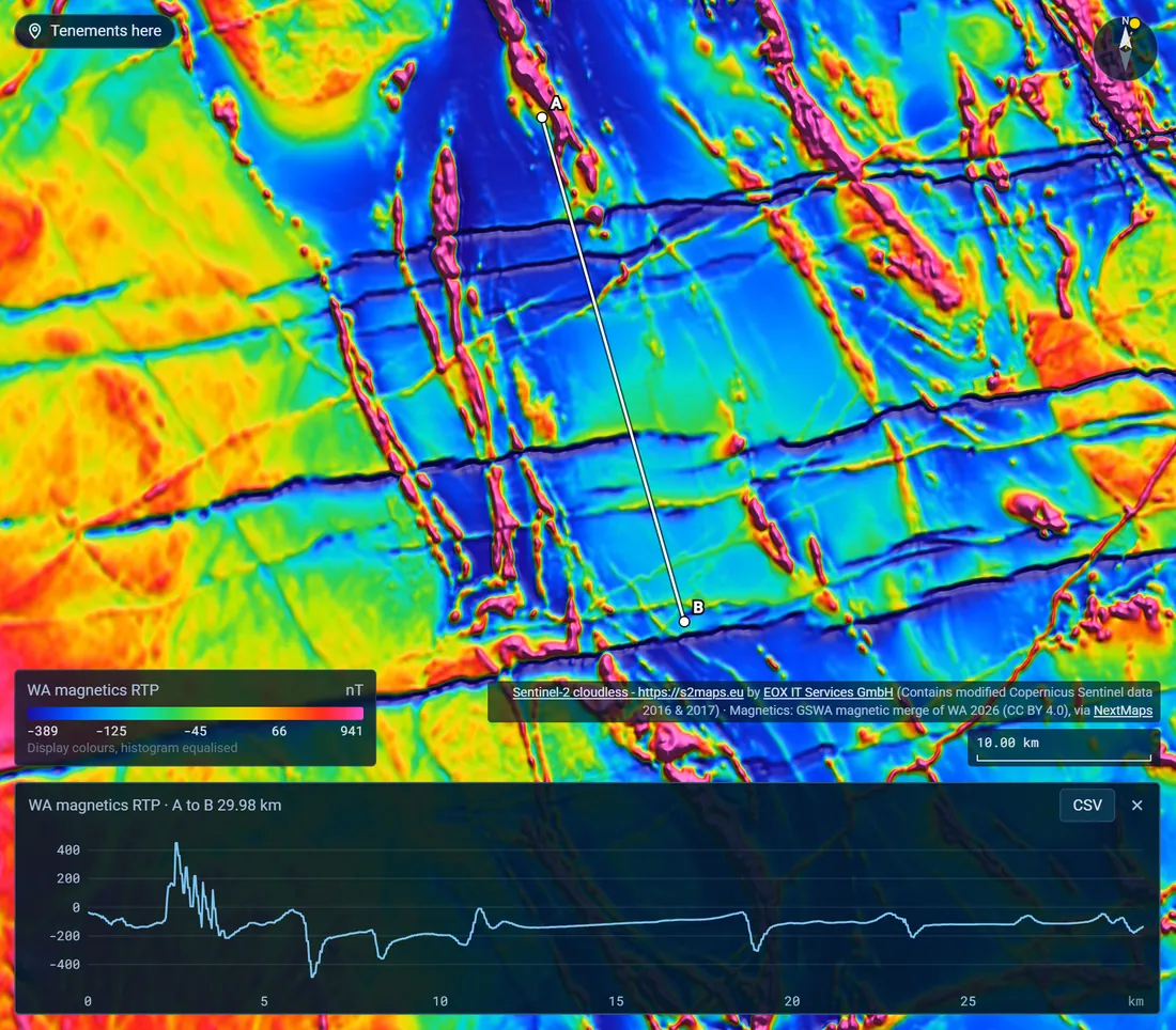
Signs that remanence is at work: an anomaly that stays a low or a lopsided pair after RTP, one that does not fit the mapped geology, or a body whose anomaly suggests a different shape from its outline. Ways to check it: the analytic signal, which depends much less on the direction of magnetisation (it is fully independent of it only in two dimensions), drilling, and oriented samples measured for their remanence.
Derivatives, tilt and upward continuation
Filters change what the grid emphasises. None adds information: each trades one kind of detail for another.
- First vertical derivative (1VD). How fast the field changes with height. It sharpens shallow sources and their edges and suppresses broad, deep ones, which makes it the usual grid for mapping. It sharpens noise too, so flight-line stripes and culture come up with the geology.
- Second vertical derivative. Sharper and noisier again, for thin, shallow units in a well-flown survey.
- Tilt angle. The vertical derivative against the horizontal gradient, as an angle from minus 90 to plus 90 degrees. Weak and strong anomalies get the same range, so a faint unit beside a strong one shows as clearly, and the zero line tends to follow the edges of steep bodies.
- Analytic signal. Peaks over the edges of magnetic bodies, and depends less on the direction of the field and of the magnetisation than the TMI does, which helps near the equator and where remanence is strong.
- Upward continuation. Recalculates the grid as if flown higher. Shallow detail fades and broad, deep sources remain, so comparing heights separates the near surface from the deep, and tames a noisy grid.
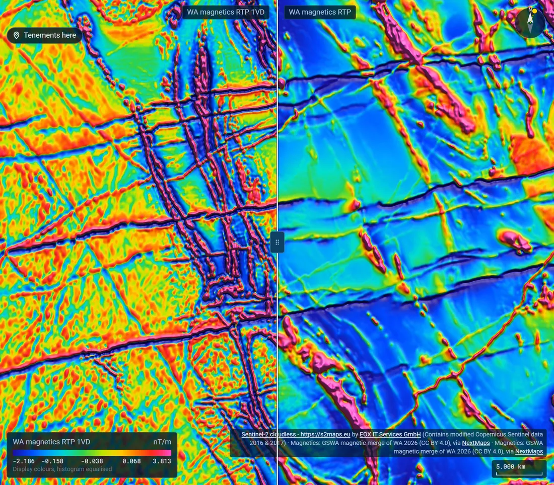
See GSWA's reduced-to-pole magnetics near Kalgoorlie with its tilt angle in Lightbox: Kalgoorlie, RTP and tilt.
Reading the structure
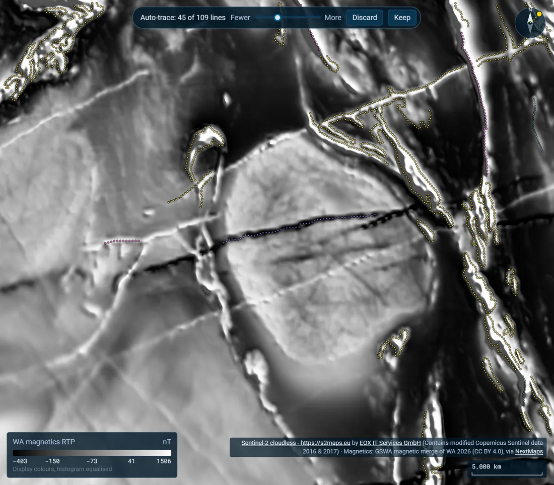
With a good display and a sharpened grid, structure reads from shapes, and from what cuts what.
- Dykes are long, narrow, straight anomalies, highs or lows, that cut across everything around them. They are often the youngest features on the grid.
- Faults show where units stop, step sideways or change character along a line. Count an offset only where the same unit can be matched on both sides: a step in one unit can be a fold or an original edge.
- Shear zones often read as linear lows where alteration destroyed the magnetite, with the units on either side dragged into them.
- Folds show in the form lines, the trends of magnetic layering, which curve around the closures. The map pattern alone does not say which way a fold closes: dips tell an antiform from a synform, and younging an anticline from a syncline.
- Contacts between units show as gradients, or as a change of texture from one domain to the next.
Put the structures in order by what cuts what, and note what cannot be told. An interpretation that says where it is uncertain is more use than one that only looks finished.
Check it against the geology
Magnetics is at its best read with everything else you know. Lay the mapped geology over the grid: units that match their magnetic domains confirm the map, and units that do not are worth a closer look, because either the mapping or the magnetics is telling you something new. Under cover the magnetics is often the best map there is, which is exactly when to be careful with rock names.
A handheld susceptibility meter on outcrop or drill core tells you which rocks actually carry the magnetite, and turns a guess about an anomaly's source into a measurement.

Know what the survey can see
- Line spacing sets the smallest feature the grid can resolve across the lines. A body narrower than the spacing may show on one line or on none, and features running along the lines are served worst.
- Flying height smooths everything. A survey flown at 100 m cannot show what one flown at 30 m does.
- Merged grids join surveys of different line spacing, height and age. The joins show as changes of texture along straight edges, and the detail stops where the finer survey does.
- Stripes along the flight lines are levelling errors, not geology. Filters can take them out, and can take out real features that run exactly along the lines with them.
- Culture, such as powerlines, pipelines, fences, railways and buildings, makes anomalies of its own: usually sharp, straight or isolated, and lined up with something on the satellite image.
Before reading detail, find out which survey you are looking at: its line spacing, height and year.
Rough depths
The magnetics gives a first estimate of how deep a source lies: enough to plan a hole or judge a target, not to replace the drill.
- Half-width rule. Over a thin, steep dyke, half the anomaly's width at half its height is roughly the depth to the dyke's top below the sensor. Subtract the flying height for its depth below the ground.
- Tilt-depth. Over the edge of a steep body, the distance between the tilt angle's zero and its plus or minus 45 degree lines is roughly the depth to the top (Salem and others, 2007).
- Euler depths. Euler deconvolution estimates depths across the whole grid for a structural index you choose to suit the source. The solutions scatter: trust tight clusters that line up along structures.
- Inversions. A 3D model that fits the data is one of many that would. Ask what constrained it, and how its depth and dip change when the constraints do.
Further reading
- Gunn, P.J., Maidment, D. and Milligan, P.R., 1997. Interpreting aeromagnetic data in areas of limited outcrop. AGSO Journal of Australian Geology and Geophysics 17(2), 175-185.
- Gunn, P.J. and Dentith, M.C., 1997. Magnetic responses associated with mineral deposits. AGSO Journal of Australian Geology and Geophysics 17(2), 145-158.
- Isles, D.J. and Rankin, L.R., 2013. Geological Interpretation of Aeromagnetic Data. Australian Society of Exploration Geophysicists.
- Li, X., 2006. Understanding 3D analytic signal amplitude. Geophysics 71(2), L13-L16.
- Li, X., 2008. Magnetic reduction-to-the-pole at low latitudes: observations and considerations. The Leading Edge 27(8), 990-1002.
- Miller, H.G. and Singh, V., 1994. Potential field tilt: a new concept for location of potential field sources. Journal of Applied Geophysics 32, 213-217.
- Reid, A.B., Allsop, J.M., Granser, H., Millett, A.J. and Somerton, I.W., 1990. Magnetic interpretation in three dimensions using Euler deconvolution. Geophysics 55(1), 80-91.
- Salem, A., Williams, S., Fairhead, J.D., Ravat, D. and Smith, R., 2007. Tilt-depth method: a simple depth estimation method using first-order magnetic derivatives. The Leading Edge 26(12), 1502-1505.